Folks,
It is accepted as fact by everyone that I know that 2/3rd of all SMT defects can be traced back to the stencil printing process. A number of us have tried to find a reference for this posit, with no success. If any reader knows of one, please let me know. Assuming this adage is true, the right amount of solder paste, squarely printed on the pad is a profoundly important metric.
In light of this perspective, some time ago, I wrote a post on calculating the confidence interval of the Cpk of the transfer efficiency in stencil printing. As a reminder, transfer efficiency is the ratio of the volume of the solder paste deposit divided by the volume of the stencil aperture. See Figure 1. Typically the goal would be 100% with upper and lower specs being 150% and 50% respectively.

Figure 1. The transfer efficiency in stencil printing is the volume of the solder paste deposit divided by the volume of the stencil aperture. Typically 100% is the goal.
I chose Cpk as the best metric to evaluate stencil printing transfer efficiencyas it incorporates both the average and the standard deviation (i.e. the “spread”). Figure 2 shows the distribution for paste A, which has a good Cpk as its data are centered between the specifications and has a sharp distribution, whereas paste B’s distribution is not centered between the specs and the distribution is broad.
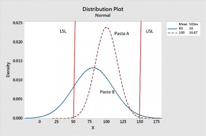
Figure 2. Paste A has the better transfer efficiency as its data are centered between the upper and lower specs, and it has a sharper distribution.
Recently, I decided to develop the math to produce an Excel spreadsheet that would perform hypothesis tests of Cpks. As far as I know this has never been done before.
An hypothesis test might look something like the following. The null hypothesis (Ho) would be that the Cpk of the transfer efficiency is 1.00. The alternative hypothesis, H1, could be that the Cpk is not equal to 1.00. H1 could also be that H1 was less than or great than 1.00.
As an example, let’s say that you want the Cpk of the transfer efficiency to be 1.00. You analyze 1000 prints and get a Cpk of 0.98. Is all lost? Not necessarily, since this was a statistical sampling, you should perform a hypothesis test. See Figure 3. In cell B16 the Cpk = 0.98 was entered, in cell B17 the sample size n = 1000 is entered, and in cell B18 the null hypothesis: Cpk = 1.00 is entered. Cell B21 shows that the null hypothesis cannot be rejected as false as the alternative hypothesis is false. So we cannot say statistically that Cpk is not equal to 1.00.
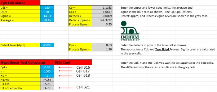
Figure 3.A Cpk = 0.98 is statistically the same as a Cpk of 1.00 as the null hypothesis, Ho, cannot be rejected.
How much different from 1.00 would the Cpk have to be in this 1000 sample example to say that it is statistically not equal to 1.00? Figure 4 shows us that the Cpk would have to 0.95 (or 1.05) to be statistically different from 1.00.

Figure 4. If the Cpk is only 0.95, this Cpk is statistically different from a Cpk = 1.00.
This spreadsheet should be useful to those who are interested in monitoring transfer efficiency Cpks to reduce end-of-line soldering defects. I will send a copy of this spreadsheet to readers who are interested. If you would like one, send me an email request to [email protected].
Cheers,
Dr. Ron