让我们去看看帕蒂和团队的情况……
几周前……
圣诞节前夕,帕蒂正从佛蒙特州伍德斯托克的家中前往常春藤大学。当她驶过图书馆时,恰巧看见伍德斯托克高中乐队正在演奏圣诞颂歌。幸运的是,附近正好有个停车位。 于是她停车下车 ,用iPhone 6S录制视频想给罗伯和孩子们看。录了几分钟后,她正要收起手机,冻僵的手指却不慎将手机摔在冰冻的水泥地上。手机就此迎来人生首个凹痕。帕蒂发出一声哀叹——苹果公司为打造最薄手机,竟让用户不得不依赖触感保护壳才能正常握持。
今天……
帕蒂正匆匆赶往办公室,她要和皮特开会。他的短信听起来很紧急。
当她快到目的地时,她查看了Fitbit® Charge和Apple Watch。她正在为常春藤大学ENGS 1《日常科技》课程的讲座比较这两款设备的健身应用。Fitbit的步数统计似乎更精准——Apple Watch会漏计非剧烈运动的步数,且无法统计爬楼梯的层数。 然而Fitbit表镜最近出现划痕(表镜竟非蓝宝石材质?),她不禁质疑:功能有限的设备售价150美元是否合理?诚然Apple Watch售价约350美元,但它能实现如此多样的功能。
当帕蒂走向办公室时,皮特正坐在外面,显得很紧张。
"怎么了?"帕蒂问道。
“我刚收到迈克·马迪根的邮件,他关于Cp和Cpk又问了些问题,”皮特回答道。
“这应该不成问题,”帕蒂回答道。
“不。但我讲Cp和Cpk就是,”皮特忧心忡忡地说。
“你一直大力宣传我在这些课题上的研究成果,还有我的Excel®电子表格,以至于沃尔特斯教授邀请我在他的统计学课堂上讲解这些内容,”皮特继续说道。
“问题是?”帕蒂问道。
“我害怕在众人面前发言,”皮特坦白道。
帕蒂停顿了一下。尽管他们共事多年,她从未见过他当众发言。接下来十分钟里,他们制定了一个计划,帮助皮特跨越这个障碍。
“你能单独和迈克谈吗?”帕蒂转移了话题。
“当然!这我能办到,”皮特立刻回道。
皮特走进办公室,重新读了一遍迈克的邮件。
Pete, thanks for your Excel spreadsheet Re Cp and Cpk. One thing we don’t understand is the difference between one-sided or two-sided defects. Can you call and chat about it? How about today at 4PM? Best, Mike.
Pete used Minitab® to develop some graphs that explained the difference between one-sided and two-sided defects. By lunchtime he was prepared for his telecon with Mike. The rest of the day went quickly as he had several meetings with students right up until his 4PM call.
下午3点59分,皮特拨通了迈克的电话。
“Hey, Pete! Thanks for calling. Our team is impressed with your Cp and Cpk spreadsheet, but we don’t understand the difference between single-sided and double-sided defects. Can you make this clear to me?” Mike began.
好的。请查看我发送的PowerPoint®幻灯片。它展示了两个孔径样本的分布情况。规格要求为1.00mm ± 0.06mm。通常我们期望规格处于3倍标准差范围内,因此标准差应为0.02mm。 注意其中一个分布的均值位于中心(1.00mm),但标准差为0.03mm,高于预期。另一个分布虽达到0.02mm的理想标准差,但均值却偏移至0.974mm。"皮特开始解释道。
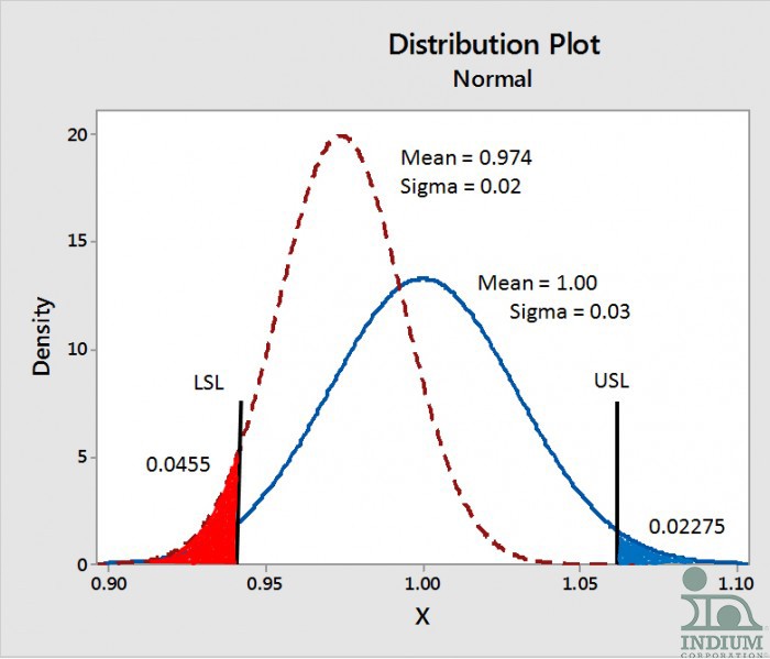
Figure: The PowerPoint® slide Pete sent to Mike. Note: for the off-centered distribution, all of the defects are below the LSL. Whereas, for the centered distribution, the defects are equal on both sides of the spec limits. The total defects are the same for bothdistributions.
“所以,其中一条曲线的 sigma 值正确,为 0.02 毫米,但偏离了中心,”迈克评论道。
他稍作停顿,接着补充道:“另一条曲线居中,但其标准差更大,达到0.03毫米。”
“Notice that all of the defects on the off-centered curve are on the low side of the spec or the lower spec limit (LSL) shown in red. Whereas, the defects on the centered curve are on both sides,” Pete continued.
“是的。我猜偏心的曲线更糟糕,尽管其标准差值较低,”迈克补充道。
“Yep. The defect rate for both is 0.0455. But, the off-center curve is worse in a manufacturing situation,” Pete responded.
“But, why is that, if the defect rate is the same?” Mike asked.
“Well, let’s say some shafts are to go into the bores. Say the shafts have a mean diameter of 0.92mm +/- 0.06. Most tolerance analysis assumes a centered distribution. The off-centered distribution of bores will have 2.8% interference fits, whereas the centered distribution will have only 1.3% interference fits, even though the sigma is 0.03mm for this distribution,” Pete elaborated.
“So, stacking all of the defects at one end can be a problem? Let me guess that the Cpk for the centered distribution is better,” Mike responded.
“是的。中心化分布的Cpk值为0.667,偏心分布的Cpk值为0.565。Cpk值确实能提供关于数据的最佳信息,”皮特总结道。
“你是怎么计算过盈配合的?”迈克问道。
“又是张Excel表格,”皮特轻笑一声。
“所以说,归根结底Cpk才是王道,对吧?”迈克问道。
“对,”皮特表示同意。
后记
帕蒂协助皮特准备了统计学课程的讲课内容,其中包括一次试讲。皮特的授课大获成功,尽管开场时有些紧张,但他很快便游刃有余。
干杯
罗恩博士